
Recurrent Neural Networks
Humans don’t start their thinking from scratch every second. As you read this essay, you understand each word based on your understanding of previous words. You don’t throw everything away and start thinking from scratch again. Your thoughts have persistence.
Traditional neural networks can’t do this, and it seems like a major shortcoming. For example, imagine you want to classify what kind of event is happening at every point in a movie. It’s unclear how a traditional neural network could use its reasoning about previous events in the film to inform later ones.
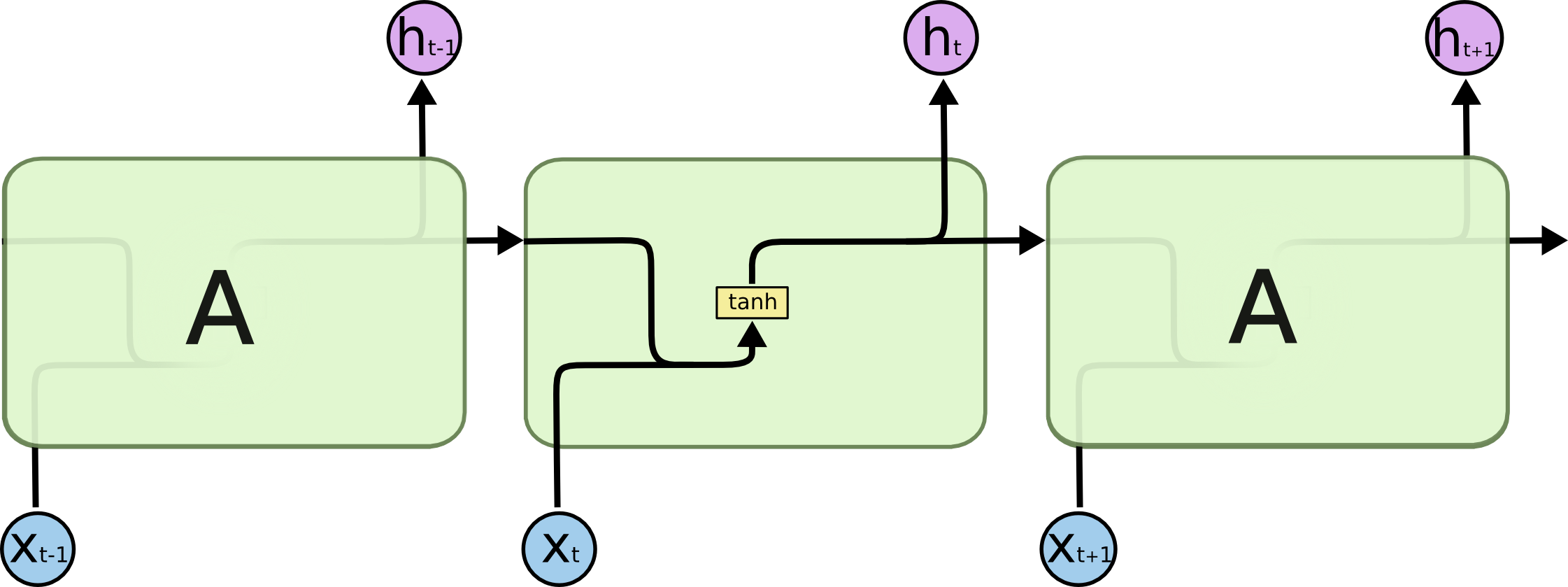
Recurrent neural networks address this issue. They are networks with loops in them, allowing information to persist.
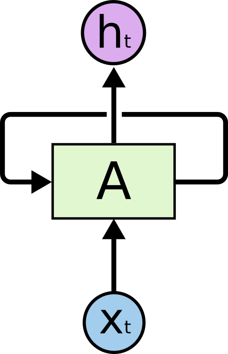
In the above diagram, a chunk of neural network, AA, looks at some input xtxt and outputs a value htht. A loop allows information to be passed from one step of the network to the next.
These loops make recurrent neural networks seem kind of mysterious. However, if you think a bit more, it turns out that they aren’t all that different than a normal neural network. A recurrent neural network can be thought of as multiple copies of the same network, each passing a message to a successor. Consider what happens if we unroll the loop:
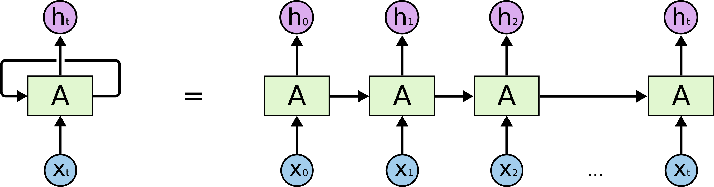
This chain-like nature reveals that recurrent neural networks are intimately related to sequences and lists. They’re the natural architecture of neural network to use for such data.
And they certainly are used! In the last few years, there have been incredible success applying RNNs to a variety of problems: speech recognition, language modeling, translation, image captioning… The list goes on. I’ll leave discussion of the amazing feats one can achieve with RNNs to Andrej Karpathy’s excellent blog post, The Unreasonable Effectiveness of Recurrent Neural Networks. But they really are pretty amazing.
Essential to these successes is the use of “LSTMs,” a very special kind of recurrent neural network which works, for many tasks, much much better than the standard version. Almost all exciting results based on recurrent neural networks are achieved with them. It’s these LSTMs that this essay will explore.
The Problem of Long-Term Dependencies
One of the appeals of RNNs is the idea that they might be able to connect previous information to the present task, such as using previous video frames might inform the understanding of the present frame. If RNNs could do this, they’d be extremely useful. But can they? It depends.
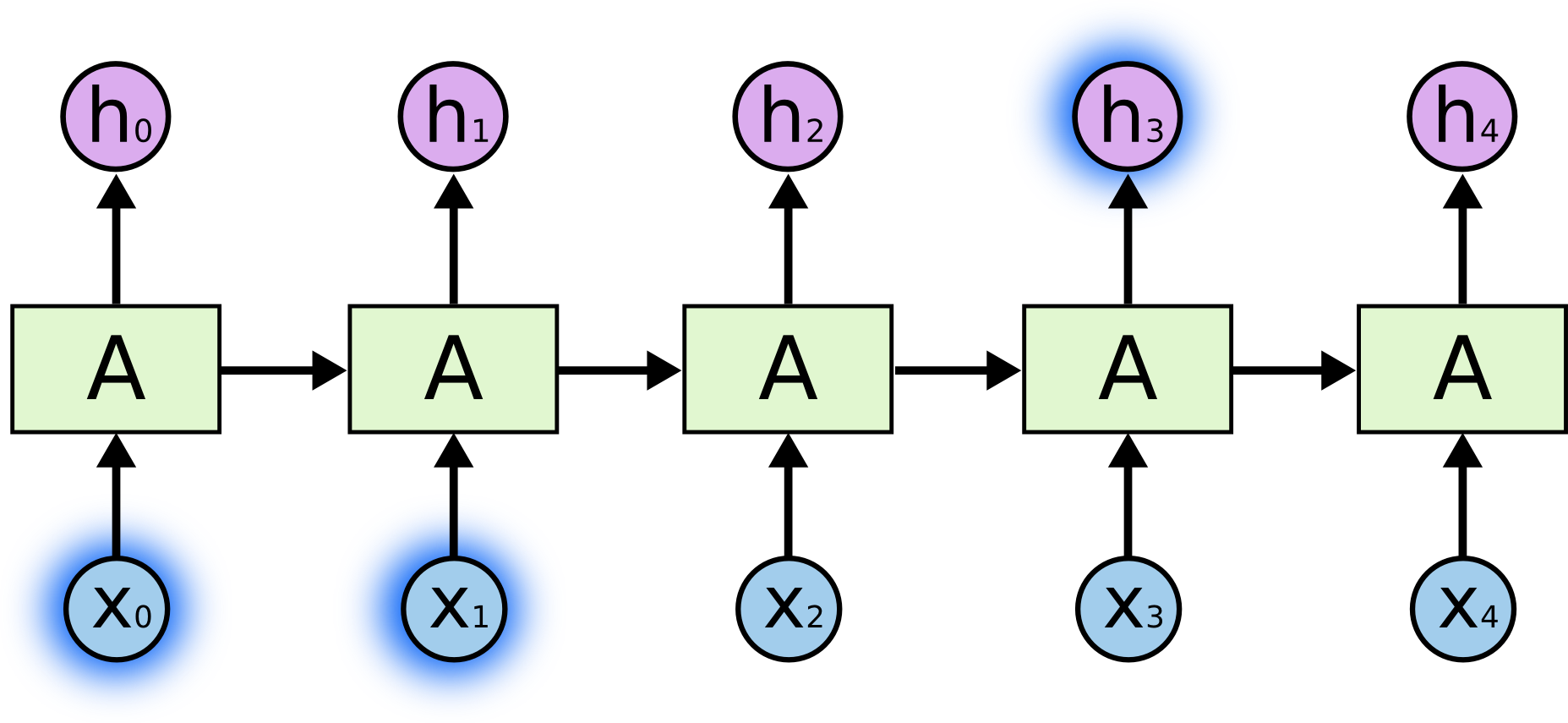
Sometimes, we only need to look at recent information to perform the present task. For example, consider a language model trying to predict the next word based on the previous ones. If we are trying to predict the last word in “the clouds are in the sky,” we don’t need any further context – it’s pretty obvious the next word is going to be sky. In such cases, where the gap between the relevant information and the place that it’s needed is small, RNNs can learn to use the past information.
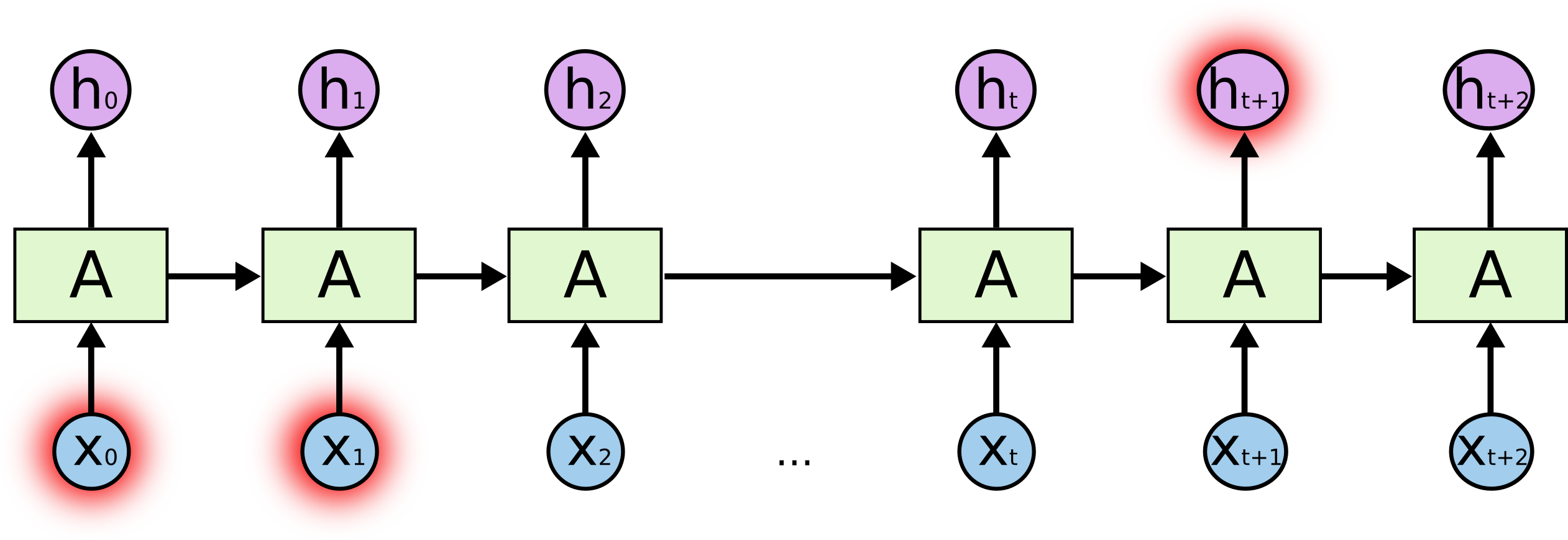
But there are also cases where we need more context. Consider trying to predict the last word in the text “I grew up in France… I speak fluent French.” Recent information suggests that the next word is probably the name of a language, but if we want to narrow down which language, we need the context of France, from further back. It’s entirely possible for the gap between the relevant information and the point where it is needed to become very large.
Unfortunately, as that gap grows, RNNs become unable to learn to connect the information.
In theory, RNNs are absolutely capable of handling such “long-term dependencies.” A human could carefully pick parameters for them to solve toy problems of this form. Sadly, in practice, RNNs don’t seem to be able to learn them. The problem was explored in depth by Hochreiter (1991) [German] and Bengio, et al. (1994), who found some pretty fundamental reasons why it might be difficult.
Thankfully, LSTMs don’t have this problem!
LSTM Networks
Long Short Term Memory networks – usually just called “LSTMs” – are a special kind of RNN, capable of learning long-term dependencies. They were introduced by Hochreiter & Schmidhuber (1997), and were refined and popularized by many people in following work.1 They work tremendously well on a large variety of problems, and are now widely used.
LSTMs are explicitly designed to avoid the long-term dependency problem. Remembering information for long periods of time is practically their default behavior, not something they struggle to learn!
All recurrent neural networks have the form of a chain of repeating modules of neural network. In standard RNNs, this repeating module will have a very simple structure, such as a single tanh layer.
LSTMs also have this chain like structure, but the repeating module has a different structure. Instead of having a single neural network layer, there are four, interacting in a very special way.

Don’t worry about the details of what’s going on. We’ll walk through the LSTM diagram step by step later. For now, let’s just try to get comfortable with the notation we’ll be using.
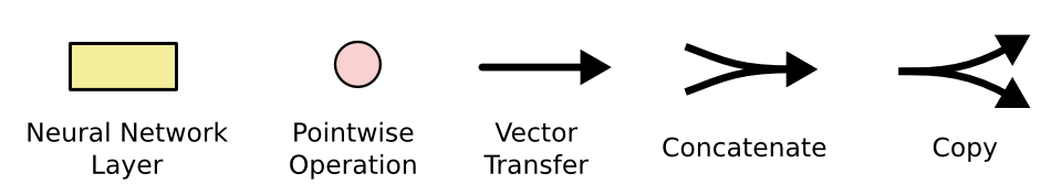
In the above diagram, each line carries an entire vector, from the output of one node to the inputs of others. The pink circles represent pointwise operations, like vector addition, while the yellow boxes are learned neural network layers. Lines merging denote concatenation, while a line forking denote its content being copied and the copies going to different locations.
The Core Idea Behind LSTMs
The key to LSTMs is the cell state, the horizontal line running through the top of the diagram.
The cell state is kind of like a conveyor belt. It runs straight down the entire chain, with only some minor linear interactions. It’s very easy for information to just flow along it unchanged.
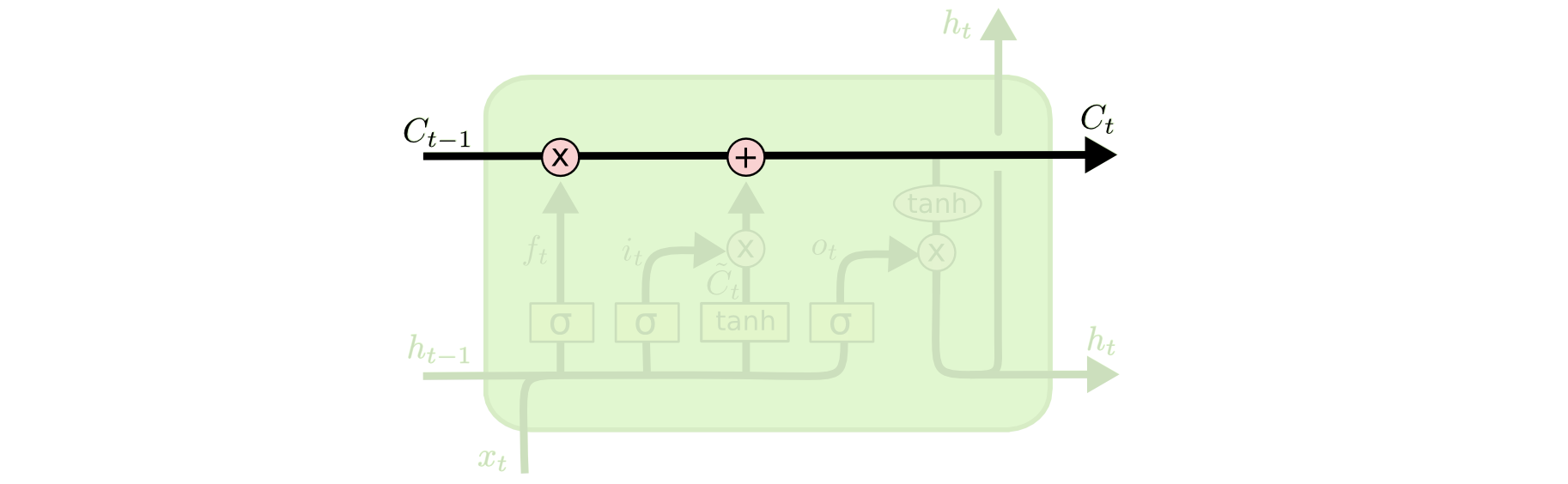
The LSTM does have the ability to remove or add information to the cell state, carefully regulated by structures called gates.
Gates are a way to optionally let information through. They are composed out of a sigmoid neural net layer and a pointwise multiplication operation.
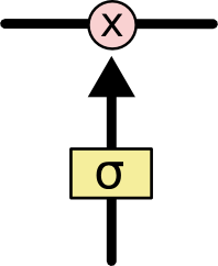
The sigmoid layer outputs numbers between zero and one, describing how much of each component should be let through. A value of zero means “let nothing through,” while a value of one means “let everything through!”
An LSTM has three of these gates, to protect and control the cell state.
Step-by-Step LSTM Walk Through
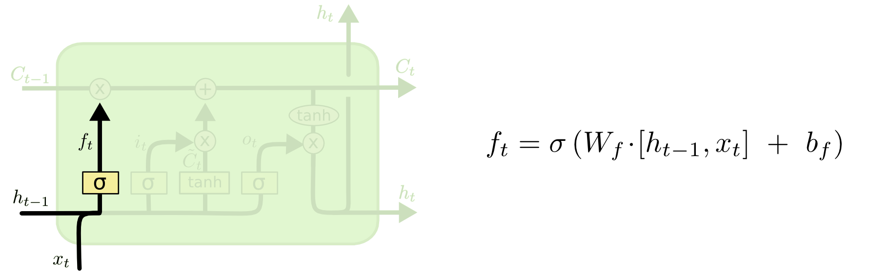
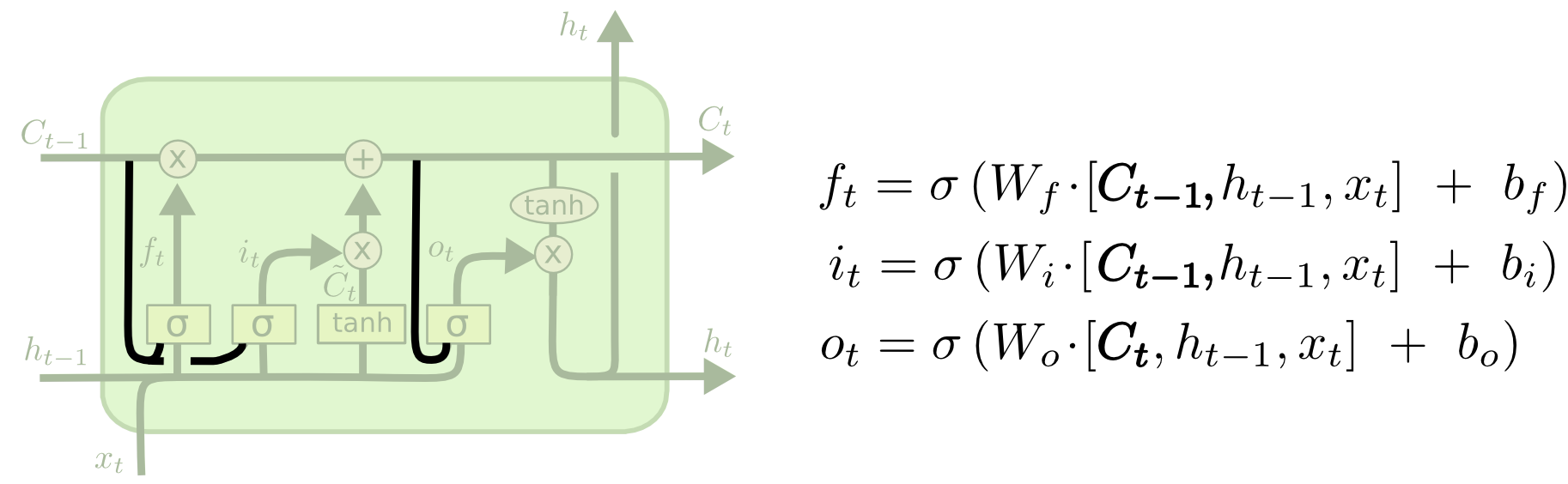
The first step in our LSTM is to decide what information we’re going to throw away from the cell state. This decision is made by a sigmoid layer called the “forget gate layer.” It looks at ht−1ht−1 and xtxt, and outputs a number between 00 and 11 for each number in the cell state Ct−1Ct−1. A 11 represents “completely keep this” while a 00 represents “completely get rid of this.”
Let’s go back to our example of a language model trying to predict the next word based on all the previous ones. In such a problem, the cell state might include the gender of the present subject, so that the correct pronouns can be used. When we see a new subject, we want to forget the gender of the old subject.
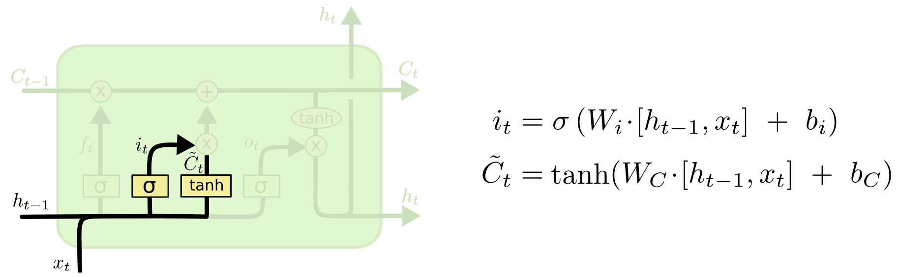
The next step is to decide what new information we’re going to store in the cell state. This has two parts. First, a sigmoid layer called the “input gate layer” decides which values we’ll update. Next, a tanh layer creates a vector of new candidate values, C~tC~t, that could be added to the state. In the next step, we’ll combine these two to create an update to the state.
In the example of our language model, we’d want to add the gender of the new subject to the cell state, to replace the old one we’re forgetting.
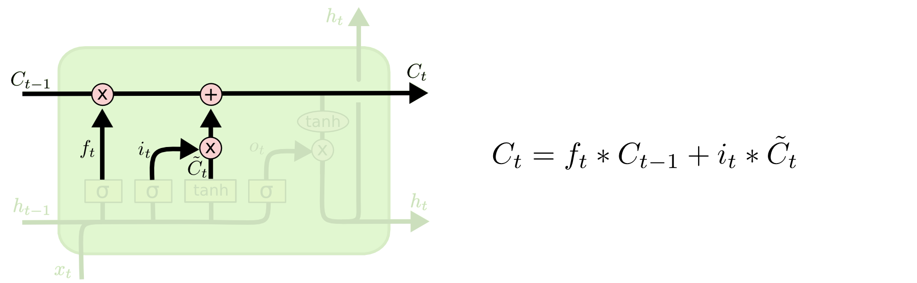
It’s now time to update the old cell state, Ct−1Ct−1, into the new cell state CtCt. The previous steps already decided what to do, we just need to actually do it.
We multiply the old state by ftft, forgetting the things we decided to forget earlier. Then we add it∗C~tit∗C~t. This is the new candidate values, scaled by how much we decided to update each state value.
In the case of the language model, this is where we’d actually drop the information about the old subject’s gender and add the new information, as we decided in the previous steps.
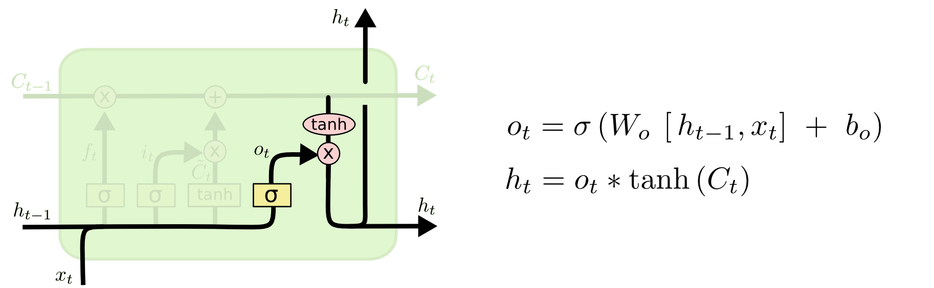
Finally, we need to decide what we’re going to output. This output will be based on our cell state, but will be a filtered version. First, we run a sigmoid layer which decides what parts of the cell state we’re going to output. Then, we put the cell state through tanhtanh (to push the values to be between −1−1 and 11) and multiply it by the output of the sigmoid gate, so that we only output the parts we decided to.
For the language model example, since it just saw a subject, it might want to output information relevant to a verb, in case that’s what is coming next. For example, it might output whether the subject is singular or plural, so that we know what form a verb should be conjugated into if that’s what follows next.
Variants on Long Short Term Memory
What I’ve described so far is a pretty normal LSTM. But not all LSTMs are the same as the above. In fact, it seems like almost every paper involving LSTMs uses a slightly different version. The differences are minor, but it’s worth mentioning some of them.
One popular LSTM variant, introduced by Gers & Schmidhuber (2000), is adding “peephole connections.” This means that we let the gate layers look at the cell state.
The above diagram adds peepholes to all the gates, but many papers will give some peepholes and not others.
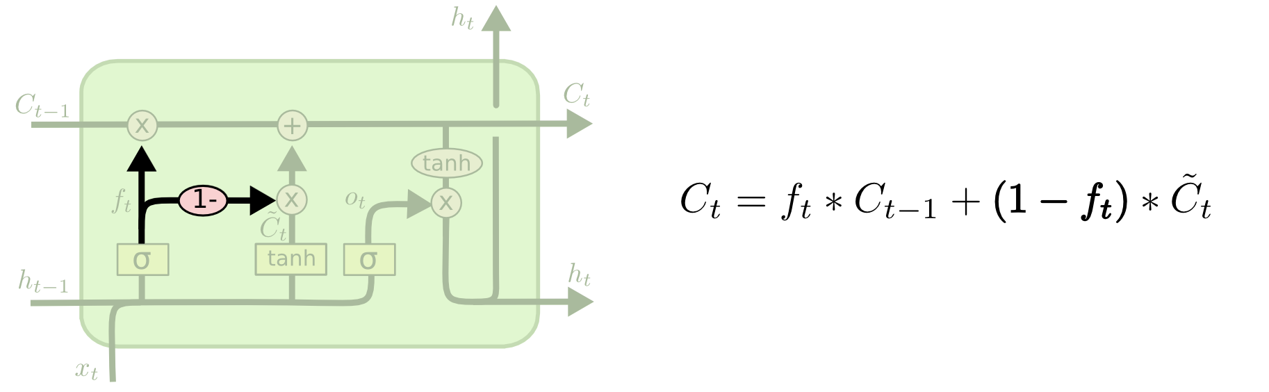
Another variation is to use coupled forget and input gates. Instead of separately deciding what to forget and what we should add new information to, we make those decisions together. We only forget when we’re going to input something in its place. We only input new values to the state when we forget something older.
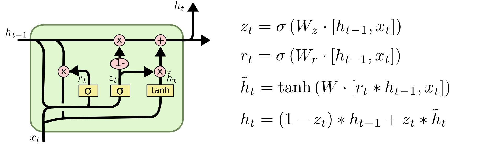
A slightly more dramatic variation on the LSTM is the Gated Recurrent Unit, or GRU, introduced by Cho, et al. (2014). It combines the forget and input gates into a single “update gate.” It also merges the cell state and hidden state, and makes some other changes. The resulting model is simpler than standard LSTM models, and has been growing increasingly popular.
These are only a few of the most notable LSTM variants. There are lots of others, like Depth Gated RNNs by Yao, et al. (2015). There’s also some completely different approach to tackling long-term dependencies, like Clockwork RNNs by Koutnik, et al. (2014).
Which of these variants is best? Do the differences matter? Greff, et al. (2015) do a nice comparison of popular variants, finding that they’re all about the same. Jozefowicz, et al. (2015)tested more than ten thousand RNN architectures, finding some that worked better than LSTMs on certain tasks.
Conclusion
Earlier, I mentioned the remarkable results people are achieving with RNNs. Essentially all of these are achieved using LSTMs. They really work a lot better for most tasks!
Written down as a set of equations, LSTMs look pretty intimidating. Hopefully, walking through them step by step in this essay has made them a bit more approachable.
LSTMs were a big step in what we can accomplish with RNNs. It’s natural to wonder: is there another big step? A common opinion among researchers is: “Yes! There is a next step and it’s attention!” The idea is to let every step of an RNN pick information to look at from some larger collection of information. For example, if you are using an RNN to create a caption describing an image, it might pick a part of the image to look at for every word it outputs. In fact, Xu, et al.(2015) do exactly this – it might be a fun starting point if you want to explore attention! There’s been a number of really exciting results using attention, and it seems like a lot more are around the corner…
Attention isn’t the only exciting thread in RNN research. For example, Grid LSTMs byKalchbrenner, et al. (2015) seem extremely promising. Work using RNNs in generative models – such as Gregor, et al. (2015), Chung, et al. (2015), or Bayer & Osendorfer (2015) – also seems very interesting. The last few years have been an exciting time for recurrent neural networks, and the coming ones promise to only be more so!
Acknowledgments
I’m grateful to a number of people for helping me better understand LSTMs, commenting on the visualizations, and providing feedback on this post.
I’m very grateful to my colleagues at Google for their helpful feedback, especially Oriol Vinyals,Greg Corrado, Jon Shlens, Luke Vilnis, and Ilya Sutskever. I’m also thankful to many other friends and colleagues for taking the time to help me, including Dario Amodei, and Jacob Steinhardt. I’m especially thankful to Kyunghyun Cho for extremely thoughtful correspondence about my diagrams.
Before this post, I practiced explaining LSTMs during two seminar series I taught on neural networks. Thanks to everyone who participated in those for their patience with me, and for their feedback.


相关推荐
一个经典的LSTM教程,以图形化方式开始,从RNN开始,逐步引入Cell的思想和各种门的思想。 Humans don’t start their thinking from scratch every second. As you read this essay, you understand each word ...
LSTM 入门经典(form Colah's blog)
Long Short Term Memory networks, usually called “LSTMs” ...understand the need of LSTM which can be explained by the drawback of practical use of Recurrent Neural Network (RNN). So, lets start with RNN
资源来源:https://colah.github.io/posts/2015-08-Understanding-LSTMs/
资源来源:https://colah.github.io/posts/2015-08-Understanding-LSTMs/
lstm introduction。LSTM基础介绍。Understanding LSTM Networks。对LSTM网络的基础内容进行介绍
中文自然语言的实体抽取和意图识别(Natural Language Understanding),可选Bi-LSTM + CRF 以上生成模型需要的语料,按1:2:13分别生成test数据、dev数据、train数据。以及用gensim生成词向量,这个可以在更大的...
Understanding Speaking Styles of Internet Speech Data with LSTM and Low-resource Training
RNN和Temporal-ConvNet进行活动识别 ,(等额缴纳) 论文代码: (在杂志上接受,2019年) 项目:...演示版GIF展示了我们的TS-LSTM和“时间-开始”方法的前3个预测结果。 顶部的文本是基本事实,三个文本是每种方法的预
Visual Question Answer (VQA) 是对视觉图像的自然语言问答,作为视觉理解 (Visual Understanding) 的一个研究方向,连接着视觉和语言。问题的格式是给定一张图片,并提出关于这张图片的问题,获得该问题的回答。 ...
话语级对话理解该存储库包含论文“”中模型的pytorch实现。任务定义给定对话的文字记录以及每个组成话语的说话者信息,话语级对话理解(话语级对话理解)任务旨在从一组预定义标签中识别每个话语的标签,这些预定义...
中文自然语言的实体抽取和意图识别(Natural Language Understanding),可选Bi-LSTM CRF 或者 IDCNN CRF
自谷歌2018年发表的《BERT: Pre-training of Deep Bidirectional Transformers for Language Understanding》,彻底摒弃了LSTM等循环网络,取得了惊人的成果。到如今,预训练语言模型(Pre-trained Language Models...
语言理解预训练 现在,针对语言理解的语言模型预训练是NLP上下文中的重要一步。 语言模型将在庞大的语料库... RNNLM,ELMo是自回归语言模型的典型示例,此存储库涵盖了单向/双向LSTM语言模型。 cf. 双向LSTM LM,ELM
Exploring an advanced state of the art deep learning models and its applications using Popular ... A mathematical background with a conceptual understanding of calculus and statistics is also desired
Some understanding of machine learning and deep learning, and familiarity with the TensorFlow framework is all you need to get started with this book. Table of Contents Chapter 1 Recognizing traffic...
DeText:深度神经文本理解框架 像树懒一样放松,让DeText为您做了解 ... CNN / BERT / LSTM用于文本编码层。 它以词嵌入矩阵为输入,并将文本数据映射为固定长度的嵌入。 值得注意的是,我们在基于交互的方法上采用
BiLSTM 84.515 84.151 模型 multinli-dev-matched multinli-dev-mismatched BiLSTM 71.075 70.555 设置 conda: conda env create -f environment.yml # To download the english tokenizer from
文字产生-tf 使用RNN和LSTM使用莎士比亚脚本创建文本生成模型。资源乔莱特·弗朗索瓦(CholletFrançois)。...” 了解LSTM网络-Colah的博客, ://colah.github.io/posts/2015-08-Understanding-LSTMs/。
关于 putput是一个为会话AI生成标记数据的库。 它使用简单,高度可定制,并且可以处理消费级笔记本电脑上的大数据生成。 putput需要几分钟的时间来设置,而要花费几秒钟的... 请注意,训练有素的LSTM可以处理现实生